This package provides tools to propagate orbital states with different methods.
Propagation is the prediction of the evolution of a system from an initial state.
In Orekit, this initial state is represented by a SpacecraftState, which is a
simple container for all needed information : orbit, mass, kinematics, attitude, date,
frame, and which can also hold any number user-defined additional data like battery
status or operating mode for example.
Propagation is based on a top level Propagation interface (which in facts extends
the PVCoordinatesProvider interface) and several implementations.
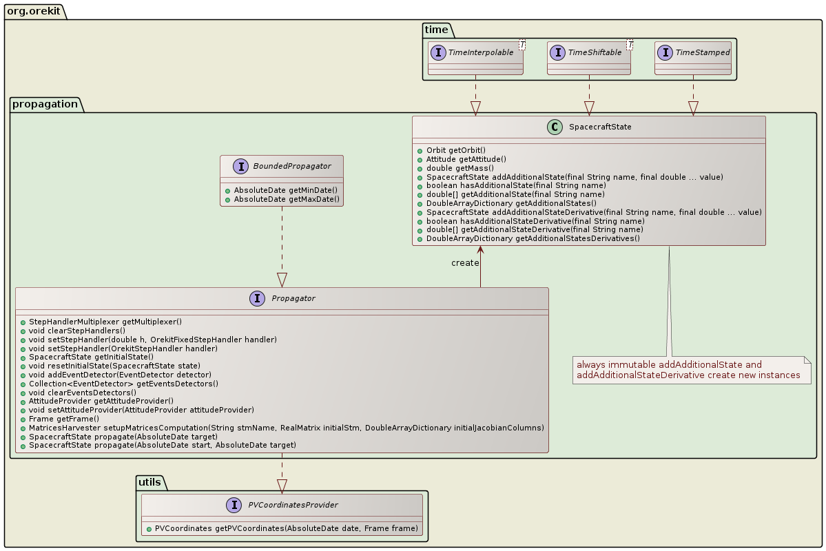
Depending on the needs of the calling application, the propagator can provide intermediate states between the initial time and propagation target time, or it can provide only the final state.
intermediate states: In order to get intermediate states, users need to register
some custom object implementation of the OrekitStepHandler or OrekitFixedStephHandler
interfaces to the propagator before running it. As the propagator computes the
evolution of spacecraft state, it performs some internal time loops and will call these
step handlers at each finalized step. Users often use this mode with only a single
call to propagation with the target propagation time representing the end final date.
The core business of the application is in the step handlers, and the application
does not really handle time by itself, it lets the propagator do it.
final state only: This method is used when the user wants to completely control the evolution of time. The application gives a target time and no step handlers at all. The propagator then has no callback to perform and its internal loop is invisible to caller application. The only feedback is the return value of the propagator with the final state at target time. Users often use this mode in loops, each target propagation time representing the next small time step.
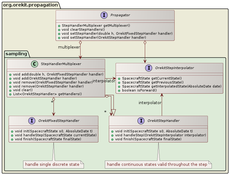
There is no limitation on the number of step handlers that can be registered to a propagator.
Each propagator contains a multiplexer that can accept several step handlers.
Step handlers can be either of OrekitFixedStepHandler type, which will be called at regular time
intervals and fed with a single SpacecraftState, or they can be of OrekitStepHandler type,
which will be called when the propagator accepts one step according to its internal time loop
(time steps duration can vary in this case) and fed with an OrekitStepInterpolator that is valid
throughout the step, hence providing dense output. The following class diagram shows this architecture.
Orekit uses this mechanism internally to provide some important features with specialized
internal step handlers. The following class diagram shows for example that the EphemerisGenerator
that can be requested from a propagator is based on a step handler that will store all intermediate
steps during the propagation. Ephemeris generation from a propagator is used when the user needs
random access to the orbit state at any time between the initial and target times, and in no
sequential order. A typical example is the implementation of search and iterative algorithms that
may navigate forward and backward inside the propagation range before finding their result.
CAVEATS: Be aware that this mode cannot support events that modify spacecraft initial state. Be aware that since this mode stores all intermediate results, it may be memory-intensive for long integration ranges and high precision/short time steps.
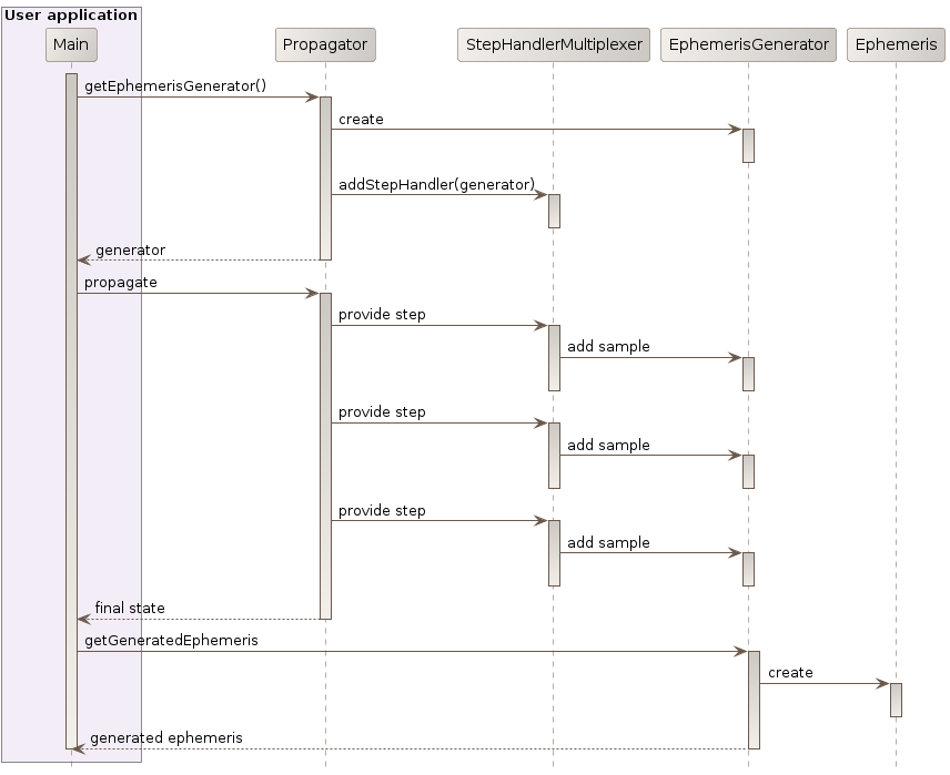
The fact ephemeris generation is based on a specialized step handler as shown in the following sequence diagram explains that in order to generate an ephemeris, users must call three methods in sequence:
final EphemerisGenerator generator = propagator.getEphemerisGenerator();
propagator.propagate(start, end);  // here we ignore the returned final state
final BoundedPropagator = generator.getGeneratedEphemeris();
Of course, as several step handlers can be used simultaneously, it is possible to generate an ephemeris and to set up other step handlers performing other computations at the same time.
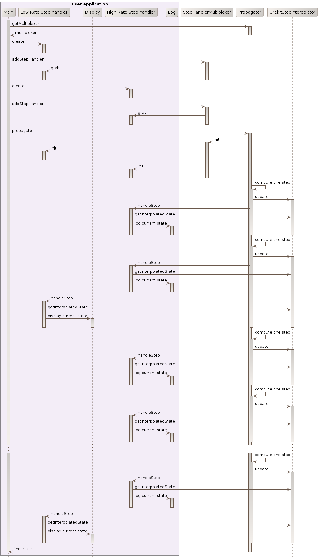
The following sequence diagram shows a use case for several step handlers dealing with fixed steps at different rates: one high rate (i.e. small step size) handler logging some detailed information on a huge log file, and at the same time a low rate (i.e. large step size) handler intended to display progress for the user if computation is expected to be long.
The next sequence diagram shows a case where users want to control the time loop tightly from within their application. In this case, the step handlers multiplexer is cleared, the propagator is called multiple time, and returns states at requested target times.
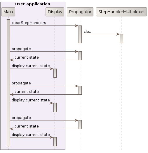
Controlling the time loop at application level by ignoring step handlers and just getting states at specified times may seem appealing and more natural to most first time Orekit users. The previous class diagram appears much simpler than the previous one. The fact is that the burden of time management complexity is on the users side, not on Orekit side. It is therefore not the recommended way to use propagation.
The recommended way is to register step handlers and call the propagation just once with the final time of the study as the target time and letting the propagator perform the time loop. It is very simple to use and allows users to get rid of concerns about synchronizing force models, file output, discrete events. All these parts are handled separately in different user code parts, and Orekit takes care of all management. From a user point of view, using step handler lead to much simpler code to maintain with smaller independent parts. Another important point is that letting the propagator manage the time loop lets it select an integration step size that may be larger than the user output sampling, which greatly increases performances (some experiments had shown up to 50 fold performance increase, mainly when high rate output are desired).
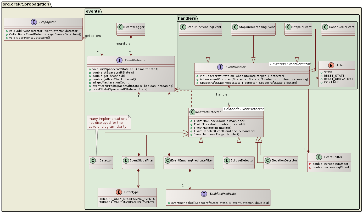
All propagators, including analytical ones, support discrete events handling during
propagation. This feature is activated by registering events detectors as defined by
the EventDetector interface to the propagator, each EventDetector being
associated with an EventHandler that will be triggered automatically at event
occurrence. The following class diagram shows the main interfaces used for event handling.
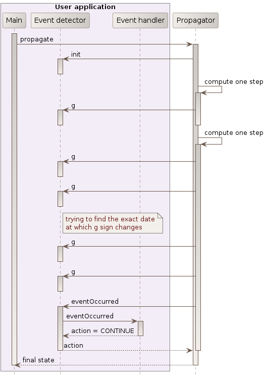
At each propagation step, the propagator checks the registered events detectors for the occurrence of some event, as shown in the following sequence diagram. If an event occurs, then the corresponding action is triggered, which can notify the propagator to resume propagation (possibly with an updated state) or to stop propagation.
Resuming propagation with changed state is used for example in the ImpulseManeuver
class. When the maneuver is triggered, the orbit is changed according to the velocity increment
associated with the maneuver and the mass is reduced according to the consumption. This
allows the handling simple maneuvers transparently even inside basic propagators like
Kepler or Eckstein-Heschler.
Stopping propagation is useful when some specific state is desired but its real occurrence
time is not known in advance. A typical example would be to find the next ascending node
or the next apogee. In this case, we can register a NodeDetector or an ApsideDetector
object and launch a propagation with a target time far away in the future. When the
event is triggered, it notifies the propagator to stop and the returned value is the state
exactly at the event time.
Users can define their own events, typically by extending the AbstractDetector abstract class.
There are also several predefined events detectors already available, amongst which :
DateDetector, which is simply triggered at a predefined date, and can be
reset to add new dates on the run (which is useful to set up delays starting when a
previous event is been detected),ElevationDetector, which is triggered at raising or setting time of a
satellite with respect to a ground point, taking atmospheric refraction into account
and either constant elevation or ground mask when threshold elevation is azimuth-dependent,ElevationExtremumDetector, which is triggered at maximum (or minimum) satellite
elevation with respect to a ground point,AltitudeDetector which is triggered when satellite crosses a predefined altitude limit
and can be used to compute easily operational forecasts,FieldOfViewDetector which is triggered when some target enters or exits a satellite
sensor Field Of View (any shape),FootprintOverlapDetector which is triggered when a sensor Field Of View (any shape,
even split in non-connected parts or containing holes) overlaps a geographic zone, which
can be non-convex, split in different sub-zones, have holes, contain the pole,GeographicZoneDetector, which is triggered when the spacecraft enters or leave a
zone, which can be non-convex, split in different sub-zones, have holes, contain the pole,GroundFieldOfViewDetector, which is triggered when the spacecraft enters or leave
a ground based Field Of View, which can be non-convex, split in different sub-zones, have holes,EclipseDetector, which is triggered when some body enters or exits the umbra or the
penumbra of another occulting body,ApsideDetector, which is triggered at apogee and perigee,NodeDetector, which is triggered at ascending and descending nodes,PositionAngleDetector, which is triggered when satellite angle on orbit crosses some
value (works with either anomaly, latitude argument or longitude argument and with either
true, eccentric or mean angles),LatitudeCrossingDetector, LatitudeExtremumDetector, LongitudeCrossingDetector,
LongitudeExtremumDetector, which are triggered when satellite position with respect
to central body reaches some predefined values,AlignmentDetector, which is triggered when satellite and some body projected
in the orbital plane have a specified angular separation (the term AlignmentDetector
is clearly a misnomer as the angular separation may be non-zero),AngularSeparationDetector, which is triggered when angular separation between satellite and
some beacon as seen by an observer goes below a threshold. The beacon is typically the Sun, the
observer is typically a ground stationAngularSeparationFromSatelliteDetector, which is triggered when two moving objects come
close to each other, as seen from spacecraftFunctionalDetector, which is triggered according to a user-supplied function, which can
be a simple lambda-expressionGroundAtNightDetector, which is triggered when at civil, nautical or astronomical
down/dusk times (this is mainly useful for scheduling optical measurements from ground telescopes)HaloXZPlaneCrossingDetector, which is triggered when a spacecraft on a halo orbit
crosses the XZ planeIntersatDirectViewDetector, which is triggered when two spacecraft are in direct view,
i.e. when the central body limb does not obstruct viewMagneticFieldDetector, which is triggered when South-Atlantic anomaly frontier is crossedParameterDrivenDateIntervalDetector, which is triggered at time interval boundaries, with
the additional feature that these boundaries can be offset thanks to parameter driversAn EventShifter is also provided in order to slightly shift the events occurrences times.
A typical use case is for handling operational delays before or after some physical event
really occurs.
An EventSlopeFilter is provided when user is only interested in one kind of events that
occurs in pairs like raising in the raising/setting pair for elevation detector, or
eclipse entry in the entry/exit pair for eclipse detector. The filter does not simply
ignore events after they have been detected, it filters them before they are located
and hence save some computation time by not doing an accurate search for events that
will ultimately be ignored.
An EventEnablingPredicateFilter is provided when user wants to filter out some
events based on an external condition set up by a user-provided enabling predicate
function. This allow for example to dynamically turn some events on and off during
propagation or to set up some elaborate logic like triggering on elevation first
time derivative (i.e. one elevation maximum) but only when elevation itself is above
some threshold. The filter does not simply ignore events after they have been detected,
it filters them before they are located and hence save some computation time by not doing
an accurate search for events that will ultimately be ignored.
A BooleanDetector is provided to combine several other detectors with boolean
operators and, or and not. This allows for example to detect when a satellite
is both visible from a ground station and out of eclipse.
A NegateDetector is provided to negate the sign of the switching function g of another detector.
Event occurring can be automatically logged using the EventsLogger class.
All propagators can be used to propagate user additional states on top of regular orbit attitude and mass state. These additional states will be available throughout propagation, i.e. they can be used in the step handlers, in the event detectors and events handlers and they will also be available in the final propagated state. There are three main cases:
AdditionalStateProvider interface and register it to the propagator, which will
call it each time it builds a SpacecraftState.AdditionalDerivativesProvider interface
and register it to an integrator-based propagator, which will integrated it and
provide the integrated state.The first two cases correspond to additional states managed by the propagator, the
last case not being considered as managed. The list of states managed by the propagator
is available using the getManagedAdditionalStates and isAdditionalStateManaged.
The following class diagram shows the available propagators
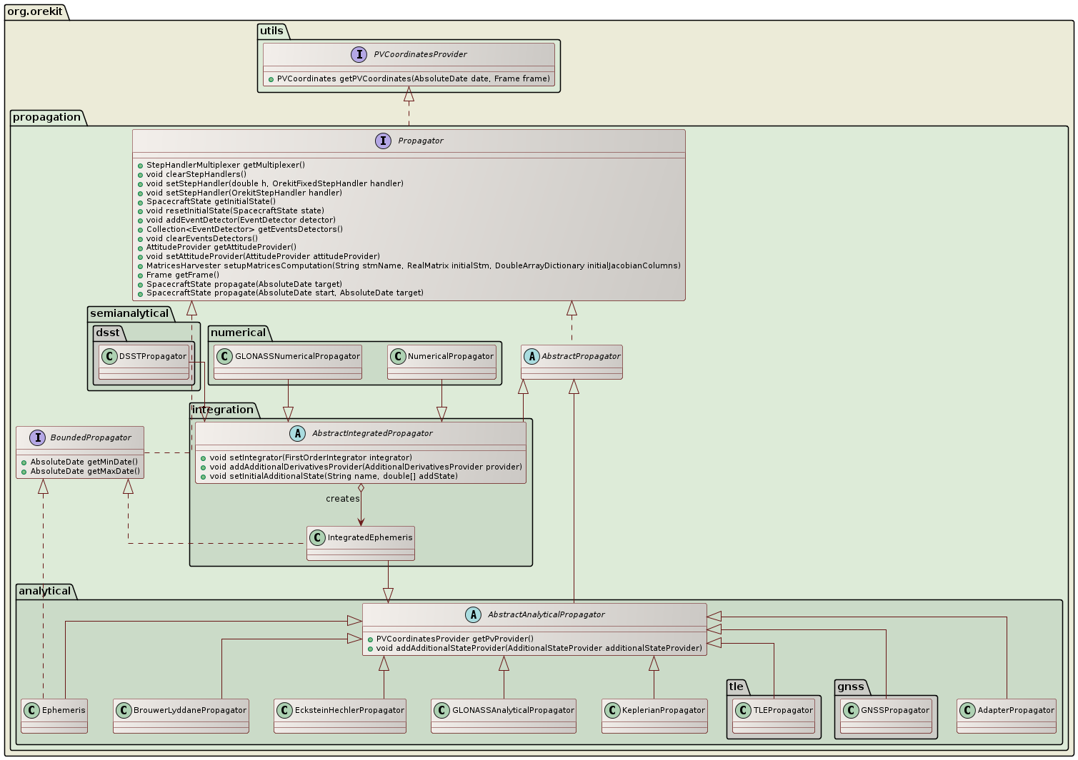
The KeplerianPropagator is based on Keplerian-only motion. It depends only on µ.
This analytical model is suited for near-circular orbits and inclination neither equatorial nor critical. It considers J2 to J6 potential zonal coefficients, and uses mean parameters to compute the new position.
Note that before version 7.0, there was a large inconsistency in the generated orbits. It was fixed as of version 7.0 of Orekit, with a visible side effect. The problem is that if the circular parameters produced by the Eckstein-Hechler model are used to build an orbit considered to be osculating, the velocity deduced from this orbit was inconsistent with the position evolution! The reason is that the model includes non-Keplerian effects but it does not include a corresponding circular/Cartesian conversion. As a consequence, all subsequent computation involving velocity were wrong. This includes attitude modes like yaw compensation and Doppler effect. As this effect was considered serious enough and as accurate velocities were considered important, the propagator now generates Cartesian orbits which are built in a special way to ensure consistency throughout propagation. A side effect is that if circular parameters are rebuilt by user from these propagated Cartesian orbit, the circular parameters will generally not match the initial orbit (differences in semi-major axis can exceed 120 m). The position however will match to sub-micrometer level, and this position will be identical to the positions that were generated by previous versions (in other words, the internals of the models have not been changed, only the output parameters have been changed). The correctness of the initialization has been assessed and is good, as it allows the subsequent orbit to remain close to a numerical reference orbit.
If users need a more definitive initialization of an Eckstein-Hechler propagator, they should consider using a propagator converter to initialize their Eckstein-Hechler propagator using a complete sample instead of just a single initial orbit.
At the opposite of the Eckstein-Hechler model, the Brouwer-Lyddane model is suited for elliptical orbits. In other words, there is no problem having a small (or big) eccentricity or inclination. Lyddane helped to solve this issue with the Brouwer model by summing the long and short periodic variations of the mean anomaly with the ones of the argument of perigee. One needs still to be careful with eccentricities lower than 5e-4. Singularity for the critical inclination i = 63.4° is avoided using the method developed in Warren Phipps' 1992 thesis.
The Brouwer-Lyddane model considers J2 to J5 potential zonal coefficients, and uses the mean and short periodic variation of the keplerian elements to compute the position. However, for low Earth orbits, the magnitude of the perturbative acceleration due to atmospheric drag can be significant. Warren Phipps' 1992 thesis considered the atmospheric drag by time derivatives of the mean mean anomaly using the catch-all coefficient M2. Usually, M2 is adjusted during an orbit determination process and it represents the combination of all unmodeled secular along-track effects (i.e. not just the atmospheric drag). The behavior of M2 is close to the B* parameter for the TLE.
There are several dedicated models used for GNSS constellations propagation. These models are generally fed by navigation messages or ephemerides updated regularly or directly from the satellites signals. All naviagation constellations are supported (GPS, Galileo, GLONASS, Beidou, IRNSS, QZSS and SBAS).
This analytical model is dedicated to Two-Line Elements (TLE) propagation.
This model is used to add to an underlying propagator some effects it does not take into account. A typical example is to add small station-keeping maneuvers to a pre-computed ephemeris or reference orbit which does not take these maneuvers into account. The additive maneuvers can take both the direct effect (Keplerian part) and the induced effect due for example to J2 which changes ascending node rate when a maneuver changed inclination or semi-major axis of a Sun-Synchronous satellite.
Numerical propagation is one of the most important parts of the Orekit project.
Based on Hipparchus ordinary differential equations integrators, the
NumericalPropagator class realizes the interface between space mechanics and
mathematical resolutions. Despite its utilization seems daunting on first sight,
it is in fact quite straigthforward to use.
The mathematical problem to integrate is a dimension-seven time-derivative equations
system. The six first elements of the state vector are the orbital parameters, which
may be any orbit type (KeplerianOrbit, CircularOrbit, EquinoctialOrbit or
CartesianOrbit) in meters and radians, and the last element is the mass in
kilograms. It is possible to have more elements in the state vector if AdditionalDerivativesProvider
have been added (this is used for example by internal classes that implement AdditionalDerivativesProvider
in order to compute State Transition Matrix and Jacobians matrices with respect to propagation
parameters). The time derivatives are computed automatically by the Orekit using the Gauss
equations for the first parameters corresponding to the selected orbit type and the flow rate
for mass evolution during maneuvers. The user only needs to register the various force models needed
for the simulation. Various force models are already available in the library and specialized
ones can be added by users easily for specific needs.
The integrators (first order integrators) provided by Hipparchus need the state vector at t0, the state vector first time derivative at t0, and then calculates the next step state vector, and asks for the next first time derivative, etc. until it reaches the final asked date. These underlying numerical integrators can also be configured. Typical tuning parameters for adaptive stepsize integrators are the min, max and perhaps start step size as well as the absolute and/or relative errors thresholds. The following code snippet shows a typical setting for Low Earth Orbit propagation:
// steps limits
final double minStep  = 0.001;
final double maxStep  = 1000;
final double initStep = 60;

// error control parameters (absolute and relative)
final double positionError = 10.0;
final double[][] tolerances = NumericalPropagator.tolerances(positionError, orbit, orbit.getType());

// set up mathematical integrator
AdaptiveStepsizeIntegrator integrator =
    new DormandPrince853Integrator(minStep, maxStep, tolerances[0], tolerances[1]);
integrator.setInitialStepSize(initStep);

// set up space dynamics propagator
propagator = new NumericalPropagator(integrator);
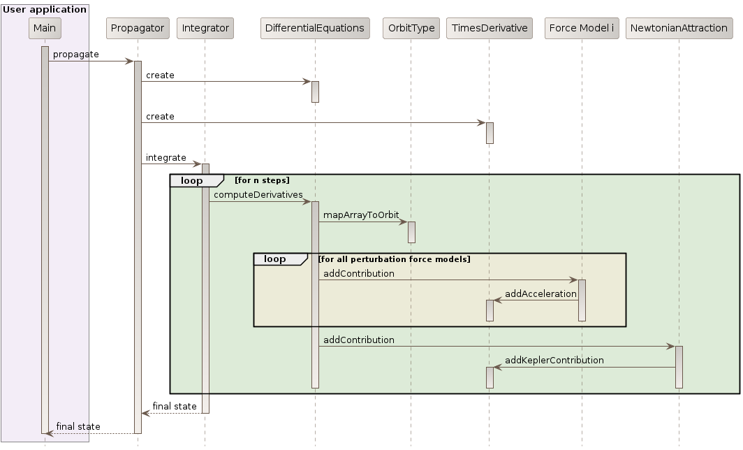
The following sequence diagram show the internal calls triggered during a numerical propagation. The important thing to note is that the force model are decoupled from the integration process, they only need to compute an acceleration.
Sometimes, simple equations of motion are not enough. Some additional parameters can be useful alongside with the trajectory, like dual parameters in optimal control or Jacobians (also called state-transition matrices). This second case especially useful for computing sensitivity of a trajectory with respect to initial state changes or with respect to force models parameters changes.
Orekit handle both cases using additional state, which can be either integrated if modeled as additional
derivatives providers (for NumericalPropagator and DSSTPropagator) or computed analytically
(for analytical propagators). When modelization requires integrating derivatives, the corresponding
equations and states are not be used for step control, though, so integrating with or without these
equations should not change the trajectory and no tolerance setting is needed for them.
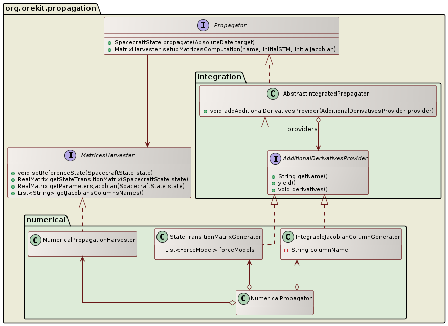
The above class diagram shows how partial derivatives are computed in the case of NumericalPropagator.
As can be seen, all propagators provide a way to trigger computation of partial derivatives
matrices (State Transition Matrix and Jacobians with respect to parameters) by providing an providing an
opaque MatrixHarvester interface users can call to retrieve these matrices from the propagated states.
Internally, NumericalPropagator references a package private implementation of this interface and uses
as well several other package private classes (StateTransitionMatrixGenerator and
IntegrableJacobianColumnGenerator to populate the matrices. The helper classes implement
AdditionalDerivativesProvider to model the matrices elements evolution and propagate both the main set
of equations corresponding to the equations of motion and the additional set corresponding to the Jacobians
of the main set. This additional set is therefore tightly linked to the main set and in particular depends
on the selected force models. The various force models add their direct contribution directly to the main
set, just as in simple propagation.
Semianalytical propagation is an intermediate between analytical and numerical propagation. It retains the best of both worlds, speed from analytical models and accuracy from numerical models. Semianalytical propagation is implemented using Draper Semianalytical Satellite Theory (DSST).
Since version 7.0, both mean elements equations of motion models and short periodic terms have been implemented and validated.
Since version 10.0 propagating both equations of motions and additional equations is available for the semianalytical propagation.
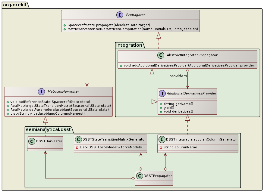
The above class diagram shows the design of the partial derivatives equations for the semianalytical propagation. As can be seen, the process is very close the one for the numerical propagation.
Since 10.0, all of the Orekit propagators have both a regular
version the propagates states based on classical real numbers (i.e. double precision numbers)
and a more general version that propagates states based on any class that implements the
CalculusFieldElement interface from Hipparchus. Such classes mimic real numbers in the way they
support all operations from the real field (addition, subtraction, multiplication, division,
but also direct and inverse trigonometric functions, direct and inverse hyperbolic functions,
logarithms, powers, roots…).
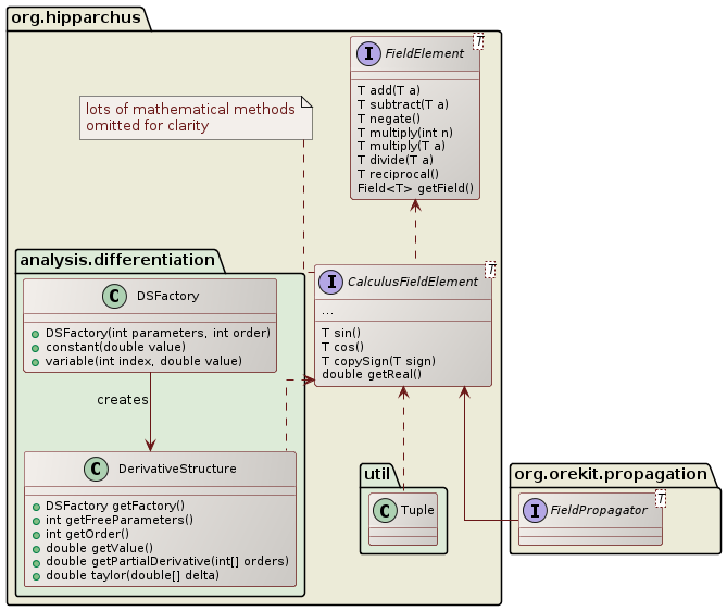
A very important implementation of the CalculusFieldElement interface is the DerivativeStructure
class, which in addition to compute the result of the canonical operation (add, multiply, sin,
atanh…) also computes its derivatives, with respect to any number of variables and to any
derivation order. If for example a user starts a computation with 6 canonical variables px,
py, pz, vx, vy, vz to represent an initial state and then performs a propagation. At the
end for all produced results (final position, final velocity but also geodetic altitude
with respect to an ellipsoid body or anything that Orekit computes), then for these results
one can retrieve its partial derivatives up to the computed order with respect to the 6
canonical variables. So if for example in a step handler you compute a geodetic altitude h,
you also have ∂³h/∂px²∂vz or any of the 84 components computed at order 3 for each value
(1 value, 6 first order derivatives, 14 second order derivatives, 56 third order derivatives).
The DerivativeStructure class also provides Taylor expansion, which allow to extrapolate
the result accurately to close values. This is an implementation of Taylor Algebra. Its two
main uses in space flight dynamics are
Orekit implementations of field propagators support all features from classical propagators: propagation modes, events (all events detectors), frames transforms, geodetic points. All propagators and all attitude modes are supported.
One must be aware however of the combinatorial explosion of computation size. For p derivation
parameters and o order, the number of components computed for each value is given by the
binomial coefficient (o+p¦p). As an example 6 parameters and order 6 implies every single
double in a regular propagation will be replaced by 924 numbers in field propagation. These
numbers are all combined together linearly in addition and subtraction, but quadratically
in multiplication and divisions. The DerivativeStructure class is highly optimized, but having
both high order and high number of parameters remains inherently costly.
Once the propagation has been performed, however, evaluating a Taylor expansion, for example in a Monte-Carlo application is very fast. So even if the propagation ends up to be for example a hundred of times slower than regular propagation, depending on the number of derivatives, the payoff is still very important as soon as we evaluate a few hundreds of points. As Monte-Carlo analyses more often use several thousands of evaluations, the payoff is really interesting.
Another important implementation of the CalculusFieldElement interface is the Tuple
class, which computes the same operation on a number of components of a tuple, hence
allowing to perform parallel orbit propagation in one run. Each spacecraft will correspond
to one component of the tuple. The first spacecraft (component at index 0) is the reference.
There is a catch, however. In many places in orbit propagations, there are conditional
statements the depend on the current state (for example is the spacecraft in eclipse
or still in Sun light). As a single choice is allowed, the outcome of the check is based
on the reference spacecraft only (i.e. fist component of the tuple) and the conditional
branch is selected according to this reference spacecraft. The spacecrafts represented by
the other components of the tuple will follow the same branch in the algorithm, even despite
they may not be in the same conditions. This means that using Tuple for orbit propagation
works only for close enough spacecrafts. This is well suited for finite differences,
formation flying or co-positioning, but this is not suited for constellations.
